Electric field of a moving particle

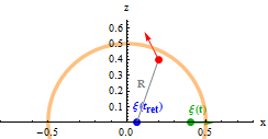
Shown is a charged sphere which is assumed to rest at the origin until time t=0. Then it is accelarated quickly to 0.8 times the speed of light. During the acceleration process, electromagnetic waves are emitted, the intensity of which is proportional to the square of the quantity of acceleration. The electromagnetic waves are not calculated, but the wave front which propagates at the speed of light is indicated by the expanding sphere, the thickness of which is a measure for the time, the accelaration process lasts.

Once the particle has the final constant velocity it generates the field which is shown inside the light sphere. Remarkably this field is directed radially in respect to the momentary position of the particle. However a field vector at a given point is generated at an earlier time. This time is called the retarded time . It is difficult to calculate because the distance between the particles position and the point is itself dependend on the retarded time: . So the equation n> is generally not solvable analytically. Here c of course is the velocity of light.

It is remarkable that the field of the moving particle is directed radially in respect to the current position beeing produced at a position much earlier during the course of the particle. This is due to the uniform motion and will be different for a non uniform movement. If the particle was moving constantly for ever then the field seen in the laboratory system would be just a Lorentz transform of a static Coulomb field, suffering a Lorentz contraction in the direction of the motion. The Lorentz contraction is indicated in the shape of the particle.
Using the phrase for ever it is sufficient that the begin of the motion is so far back in time, that the electromagnetic waves emanating from this starting time has gone far beyond the “laboratory”.

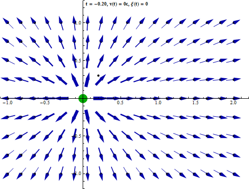
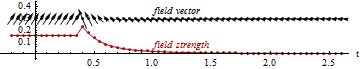
In the following diagram the development of the field at a given example point is depicted both in direction and strength over the course of time. Here the field strength is proportional to the length of the vectors whereas in the above picture the field vectors had been normalized to a certain length. The strength falls off inversely with the square of the distance so the length of the vectors would vary very much and the picture would be too confusing or the vectors far away would hardly be visible. However the strength was indicated qualitatively by the thickness of the arrows.
It is seen that in the case of instantaneous acceleration there is a discontinuity in the field strength when the information reaches the example point.

What else could happen in time

Well the charge might be accelerated actually obeying a given law, for example a uniform acceleration: v(t) = a t.
The charge might also pulsate or oscillate or move in a circle.

A simple scenario which is often used to illustrate the finite velocity of any propagation contrary to Newtons idea of instantaneous action (and hence reaction) is the narrative that “suddenly” the sun might explode and we will feel that only 8 minutes later.
A similar story might be the Gedankenexperiment that suddenly a mass or charge doubles and the action would propagate not instantaneously but with the speed of light. This is the famous “Ulrich-scenario”.
A similar example is the even more famous “Sarah-scenario”, where one charge doubles and another charge (at rest with respect to the first) in some distance simultaneously vanishes. The term “at rest” is emphasized because otherwise there would be different frames of reference to define simultaneity.

However those narratives raise certain consistency problems.
The reason is simple: These operations are not consistent with Maxwells equations.
More explicitly they contradict the very strong law of conservation of charge.
Whereas in the Sarah-scenario charge is conserved in a finite region of space - it only “jumps” mysteriously from one place to another - in the Ulrich-scenario conservation of charge is totally abandoned.
But electric charge obeyes a strong local! conservation law.
When there is a temporal change in charge at some point it has to “flow” from or to this point.
This is empirically established up to very high accuracy.
Charge is not only conserved but is also invariant with respect to different velocities (Lorentz invariance).
Then the above mentioned scenarios are nomologically impossible .
They may be metaphysically possible, but we simply don't know how to tell the story because we can't use the laws we know of.
Auf diese Gedanken hat mich eine Stelle bei Feynman gebracht.

For those who are interested in the mathematics here is the formula for the electric field at point and time t.
It is derived from the Lienard-Wiechart potentials.
  at   .
Here where is the particle position and c the velocity of light.
The coupling constant k equals in SI units.
The velocity of the particle is indicated by and is a normalized vector from the particle position to the point .
The first part in the brackets refers to the (quasi static) field, it falls off with as the Coulomb law.
The second part refers to propagating electromagnetic waves, it falls off with so the intensity falls off with .
It is essentially the term which leads for constant to the effect, that the field is directed radially to the position of the particle
at time t, whereas the field is generated at the earlier time .